Article
Summary
This post is about writing a piecewise function as a single equation, using more conventional-algebraic functions than the usual Heaviside step function. Specifically it describes a way of condensing continuous piecewise functions into a single equation using only the absolute value function (which can be written out of conventional functions).
Code
The scripts can be found at this repository, check the readme there for more info.
#1: Heaviside, and constructing our function from parts
I’ll briefly describe how to use the Heaviside step function to do it, because my solution works in a similar way.
The Heaviside step function is defined as follows:
Using it we can create the boxcar function, which is only equal to 1 over a certain interval:
(We can also create boxcar functions which go off to infinity:)
(and similar functions exist which include/exclude the endpoints, though we don’t have to worry about it for this example). Then we take our piecewise function and split it into parts:
And we multiply each part by the boxcar function over its interval:
Simplifying gives the final equation:
The colours show how the function is made up of slice functions which contain each of the component functions over a certain interval. Our approach will be to create something like these slice functions, without using weird functions like the Heaviside step function.
#2: Continuous, flat slices
Though the Heaviside method produces slices which become 0 outside of their interval, it’s enough to have slices which are constant outside of their interval.
Let me notate as a slice function which is constant at to the left and constant at to the right. Say we wanted to add another slice, to the right of it.
- For to not affect ‘s position, we have to subtract from . .
- But for to not affect ‘s position, .
Therefore only slice functions that match up in this way , , , … can be connected. However, this doesn’t say anything about the actual function piece, which can jump from to wherever it needs to go, then connect/jump back to when finished, so long as we’re able to represent such a slice function within our constraints. I’ll only consider continuous slices for now to keep things simple.
So we can join together constant slices by doing the following:
- Sort them ascending by x-position.
- Adjust each slice to start at , besides the first one.
#3: The absolute value function
I ended up looking at the absolute value for two reasons. First, you can make this almost step function:
Second, you can write it entirely out of “conventional” functions:
That makes it a prime candidate for this problem.
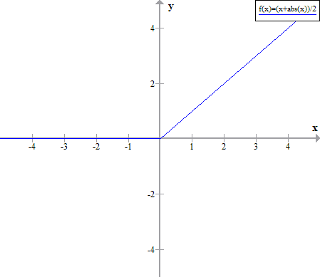
#4: The ramp and incline functions
After playing around with the absolute value function a bit, I found two functions which proved to be useful. The ramp function is a function which is constant on one end, and a line on the other:
- when , the and cancel each other out.
- when , they add together to make a line of slope 2, so we divide by 2 to normalize the line’s slope to 1.
And by staggering two ramp functions, we can create something I call the incline function, which is constant on both ends.
- when , both ramps are 0 so the result is 0.
- when , one ramp function is increasing while the other stays flat, creating a line.
- when , the ramp functions cancel each other out, keeping it constant.
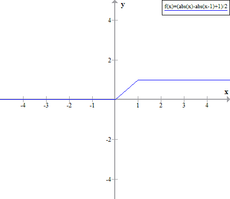
This form of the incline function generates a line segment from (0,0) to (1,1). Through translation and scaling we can create incline functions from any points (a,b) to (c,d):
- Incline from (0,0) to (1,1) =
- Incline from (a,b) to (a+1,b+1) =
- Incline from (a,b) to (a+(c-a),b+(d-b)) =
Similarly, is a “right” ramp around (0,0) with slope 1 (the line appears to the right of the point). We can scale it like so:
- Right ramp around (0,0) with slope 1:
- Right ramp around (0,0) with slope n:
- Right ramp around (a,b) with slope n:
- Left ramp around (0,0) with slope 1:
- Left ramp around (a,b) with slope n:
#5: Constructing slices
Surprisingly (dissapointingly) it’s only one easy trick from the incline function to a slice of any function we want.
To motivate it a bit, say we did have a slice of from . For this function to be continuous and flat on both ends, it would have to remain at for , and at for .
But the value plugged into looks suspiciously like an incline function — and if we set to be the incline function from (a,a) to (b,b) and plug it into , we get the function we want:
If , we would use a left ramp around (b,b) with slope 1.
If , we would use a right ramp around (a,a) with slope 1.
If both are infinity, then just use (nothing gets changed).
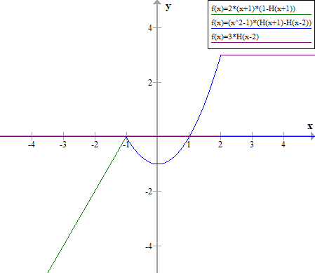
Example
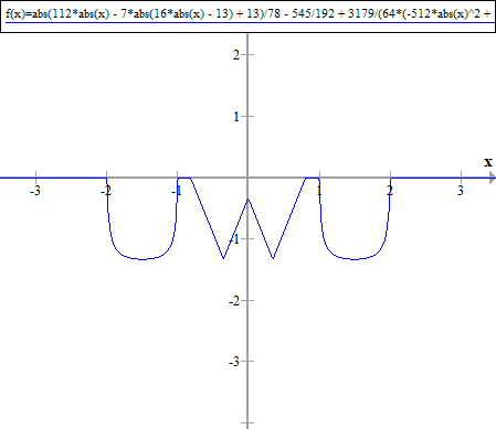
Let’s try the same function from the Heaviside example:
Create our inclines:
- = Left ramp around (-1,-1) with slope 1 =
- = Incline from (-1,-1) to (2,2) =
- = Right ramp around (2,2) with slope 1 =
Create and connect together the slices:
Simplifying:
For fun, rewriting the absolute values using square roots:
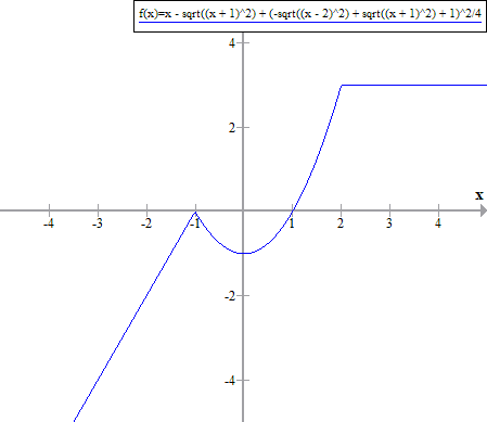
Graph of
Success!
Bonus stuff
Introducing discontinuities
So far we’ve only been working with continuous piecewise functions, but is it also possible to do this with discontinuous piecewise functions?
The way we construct our slices from functions will allow for discontinuities within the function (for example, we can construct a slice of on ). However I don’t think it’s possible to have jump discontinuities between the pieces, for the following reason:
Say we had a function with 1 or more of these discontinuities, and there was a way to write it under our constraints. We can remove all of the discontinuities by shifting the pieces around to get . now has no discontinuities between its pieces, so we can use our algorithm to find an equation for it. But now consider . This would be some sort of step function, and we would have just found a representation of it following our constraints. I don’t know how to prove that such a representation doesn’t exist, but I can’t find any evidence saying that it does, leading me to believe that it’s impossible.
Unless there is a function with a naturally occuring jump discontinuity, I don’t believe it’s possible to create piecewises containing jump discontinuities using this method.
Undefined slices
We can create slices which are undefined over a certain interval by leveraging the function , which is undefined between and 0 at . Slicing it between gives us
Running this through our algorithm above and simplifying, we can nicely write this as
If we wanted to make a single point undefined, we can use slice functions like , , …
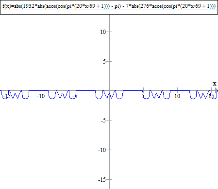
Periodic piecewise functions
Is there a trick we can use to create periodic piecewise equations?
After searching around I found a couple of interesting functions:
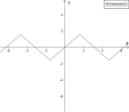
- is a linear function which oscillates between with period . This is actually listed on the Wikipedia article for triangle waves. is similar, oscillating between instead.
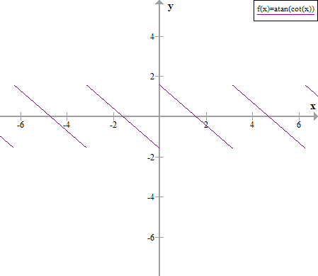
- The wikipedia page for sawtooth waves also lists the function . However this function is undefined at each multiple of , so it doesn’t work well enough for our purposes.
Ideally we’d like a sawtooth shape for our periodic functions, but I can’t find one and I have a hunch that there isn’t one based on the problems encountered with discontinuities. As far as I know there are no other elementary periodic functions besides the trigonometric ones, so any search for more periodic functions would have to involve a trigonometric term. Combining two continuous functions (+, -, x, / by nonzero, composition) will always gives you a continuous function, so a discontinuous function would also have to be involved (sqrt, log, 1/x, tan, asin, acos).
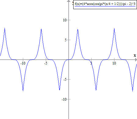
For now, we can only make oscillating periodic functions. By exchanging with and performing some other transformations, we can make an oscillating version of , where within gets mapped to in the output (see the source code for details).
Conclusion
Thanks for reading!
f(x) = abs(112*abs(x) - 7*abs(16*abs(x) - 13) + 13)/78 - 545/192 + 3179/(64*(-512*x^2 + 1536*abs(x) + 512*abs((abs(x) - 2)*(abs(x) - 1)) - 991))
f(x) = abs(1932*abs(acos(cos(pi*(20*x/69 + 1))) - pi) - 7*abs(276*acos(cos(pi*(20*x/69 + 1))) - 211*pi) + 65*pi)/(390*pi) - 545/192 + 79475*pi^2/(-1024*(69*acos(-cos(20*pi*x/69)) - 49*pi)^2 - 1024*(69*acos(-cos(20*pi*x/69)) - 29*pi)^2 + 2048*abs((69*acos(-cos(20*pi*x/69)) - 49*pi)*(69*acos(-cos(20*pi*x/69)) - 29*pi)) + 462400*pi^2)